Modelling Hydrological Impact of Climate Change on Lake Hawassa Watershed, Southern Ethiopia

Wendmagegn Girma; Brook Abate

doi:doi:10.11648/j.ijdsa.20251105.13

Research Article |

| Peer-Reviewed

Modelling Hydrological Impact of Climate Change on Lake Hawassa Watershed, Southern Ethiopia

Wendmagegn Girma^*

, Brook Abate

Published in International Journal of Data Science and Analysis (Volume 11, Issue 5)

Received: 12 September 2025 Accepted: 24 September 2025 Published: 9 October 2025

Views: Downloads:

Download PDF

Share This Article

Twitter
Linked In
Facebook

Abstract

Climate change refers to variations in the mean state of climate or variability of its properties such as rate, range and magnitude that extends for a long period due to external influences. The sign of climate change and its impact is revealing on different natural and manmade systems directly or indirectly. In this study, hydrological impact of climate change on Lake Hawassa water balance components was estimated in response to the A2a and B2a emission scenarios. Hydrological impact of climate change on Lake Hawasa water balance components were estimated in response to the A2a and B2a emission scenarios. Observed and future climatic variables were used to verify the hydrological impact. The future climate variables were predicted by using General Circulation Model (GCM) which is considered as the most used tool for estimating the future climatic condition. Statistical Downscaling Model (SDSM) was applied in order to downscale the climate variables to watershed level. Then, hydrological model soil and water analysis tool (SWAT) was applied to simulate the water balance components and calibrated by SWAT CUP (calibration uncertainty program) with sequential Uncertainty Fitting, Version 2 (SUFI-2) algorithm. The simulation result revealed that, by 2020s, the total average annual inflow volume into Lake Hawassa will rise significantly up to 6.14% for A2a and 5.9% for B2a-scenarios.

Published in	International Journal of Data Science and Analysis (Volume 11, Issue 5)
DOI	10.11648/j.ijdsa.20251105.13
Page(s)	143-152
Creative Commons	This is an Open Access article, distributed under the terms of the Creative Commons Attribution 4.0 International License (http://creativecommons.org/licenses/by/4.0/), which permits unrestricted use, distribution and reproduction in any medium or format, provided the original work is properly cited.
Copyright	Copyright © The Author(s), 2025. Published by Science Publishing Group

Keywords

Climate Change, General Circulation Model (GCM), SDSM, SWAT Hydrological Model, SWAT-CUP, SUFI 2 Algorithm

1. Introduction

Climate change refers to variations in the mean state of climate or variability of its properties such as rate, range and magnitude that extends for a long period due to external influences. Changes in solar radiation and volcanism, occur naturally and contribute to the natural variability of the climate system and the change in the composition of the atmosphere also began with the industrial revolution and the result of human activity

[1]

The IPCC (Intergovernmental Panel on Climate Change) scenarios project temperature rises of 1.4-5.8°C, and sea level rises of 9-99 cm by 2100

[2]

. Warming and precipitation are expected to vary considerably from region to region. Changes in climate average and the changes in frequency and intensity of extreme weather events are likely to have major impact on natural and human systems

[3]

Climate affects all aspects of the hydrologic cycle namely rainfall, runoff and evaporation. Changes in these components in turn affect the water availability and variability. In general, changes in climatic variables causes significant change over the hydrologic water balance components

[4, 5]

In this study we specifically estimated future water balance of Lake Hawasa with respect to base period. Numerous other studies have been conducted which assess various hydrologic parameters using downscaled global circulation models (GCMs). The overall assessment made by conducting 20 hypothetical climate sensitivity scenarios is that the annual stream flow of the Eastern Nile is very sensitive to variations in precipitation and moderately sensitive to temperature changes. In addition, the modelled response of a combined temperature and precipitation change was very similar to adding the responses from the temperature change only and precipitation change only simulations

[6]

, additionally, Climate change expected to cause significant changes in streamflow and other hydrological parameters in the period between 2045-2100 in lake Tana Basin

[7]

Generally, climate change can cause significant impact on water resources by resulting in changes in the hydrological cycle as the changes on temperature and precipitation can have a direct consequence on the quantity of evapotranspiration and on both quality and quantity of the water balance components

[8]

. Therefore, it is very important to assess the expected impact on the hydrology and water resources due to expected climate changes. The main objectives were to: develop climate variability and change scenarios using historical observation of climate and projected data of climate models (HadCM3) by applying SDSM, establish a hydrologic modeling using Soil and Water Assessment Tool (SWAT) and calibrate the SWAT model for watershed hydrology using SWAT CUP (SUFI-2 algorithm) and quantify the hydrological impact based on developed climate change scenarios of this study is to quantify the hydrological impact of climate change on Lake Hawasa watershed hydrology.

2. Methods

2.1. Description of Lake Hawasa Catchment

Lake Hawasa is located at 275km south of Addis Ababa beside of Hawasa town, which is located at (6⁰ 33'-7⁰ 33' N and 38⁰ 22' - 38⁰ 29' E) in the Ethiopian Rift Valley. Lake Hawasa is a closed and located in a caldera depression. The nested Hawasa-Korbetti Caldera complex forms a giant elliptical depression of 30- wide on the Rift floor

[9]

. The Tikurewuha River at the north eastern shore is the only perennial stream flowing into Lake Hawassa (Halcrow, 2008).

Download: Download full-size image

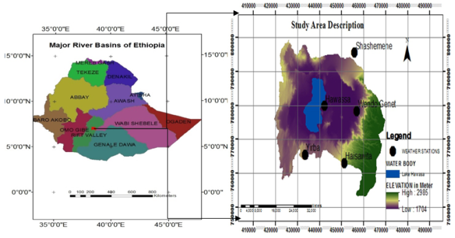
Figure 1. Location of Lake Hawasa watershed and meteorological stations.

2.2. Hydrological Impact of Climate Change

Generally, study of climate change on the hydrological regimes consists of the following three steps: The development and use of General Circulation Models (GCMs) to provide future global climate scenarios under the effect of increasing greenhouse gases, the development and use of downscaling techniques for downscaling the GCMs output to the scales compatible with hydrological models, and the development and use of hydrological models to simulate the effects of climate change on hydrological regimes at various scale

[10]

Download: Download full-size image

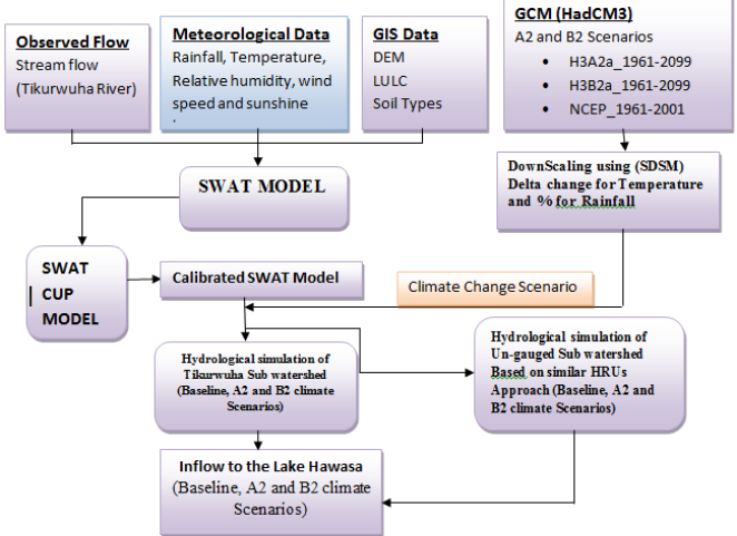
Figure 2. Overall frame work of the study.

In this study, the Global Circulation Model (GCM), Statistical Downscaling Model (SDSM) and a hydrological model (SWAT Model) were applied for the hydrological impact analysis. The overall step to study the hydrological impact of climate change was described by this simple conceptual framework shown in Figure 2.

2.3. Climate Change Scenarios and General Circulation Model (GCM)

The Special Report on Emissions Scenarios

[11, 12]

are grouped into four scenario families (A1, A2, B1 and B2) that explore alternative development pathways, covering a wide range of demographic, economic and technological driving forces and resulting greenhouse gases emissions. For this study the model output of Hadley Centre for Climate Prediction and Research Coupled Model (HadCM3) was employed for the A2 (Medium-High Emissions) and B2 (Medium-Low Emission) Scenarios. The coarse spatial resolution of the General Circulation Model (http://www.cics.uvic.ca/scenarios/sdsm/select.cgi) obtained and applied a Statistical Downscaling Model (SDSM) so as to downscale its outputs to suit the study area, therefore, the model output of HadCM3 was used in this study to simulate the climatic effect of increased atmospheric concentration of greenhouse gases and the climate model output was downscaled to catchment scale using Statistical Downscaling Model (SDSM) version 4.2.9.

The SDSM rely on empirical relationships between local-scale (predictands) and regional-scale (predictors) to downscale GCM scenarios. Compared to other downscaling methods, the statistical method is computationally inexpensive, relatively easy to use and provides station-scale climate information from GCM-scale output, which is often necessary in many climate change impact studies. During downscaling stage data quality control, screening of predictors, calibration (1978-1990) and validation (1991-2000) were performed. The impact assessments was to determine the effect of climate change with respect to the present and therefore, a 1978 to 2000 time span was selected to represent baseline period for this study. After selecting the scenarios, the future time scales from the year 2011 until 2070 were divided into two periods of 30 years considered (2011-2041 and 2041-2070).

2.4. Hydrological Model for Climate Change Study

SWAT is widely applied in many parts of the world and public domain model developed by

[13]

. It is physically based and can operate on large basins for long periods of time. SWAT simulates the hydrological cycle based on the water balance equation:

SW_t=SW_o+∑ (R_day- Q_surf- E_a- W_seep- Q_gw)(1)

Where SW_t is the final soil water content (mm), SW_o is the initial soil water content on day.

i (mm), t is the time (days), R_day is the amount of precipitation on day_i(mm), Q_surf is the amount of surface runoff on day _i (mm), Ea is the amount of evapotranspiration on day i (mm), W_seepis the amount of water entering the vadose zone from the soil profile on day i (mm), and Q_gw is the amount of return flow on day i (mm). More detailed descriptions of the different model components are listed in

[15]

The model setup begins by loading the Digital Elevation Model (DEM) and a mask of the catchments was used to focus the watershed area. The location of the Tikurwuha river gauging was added as subbasin outlet near Dato. The land use and soil map was loaded from a separate file. The hydrologic response units (HRUs) were created from the multiple land use, soil type and slope. Then, the climatic data was loaded and the interface assigned the different weather station data sets to the sub basins in the watershed. The SWAT input files were built and initial simulation performed and the model is ready to run sensitivity analysis and calibration using SWAT CUP.

Lake Hawasa obtains flow from gauged and Un-gauged sub watershed. In this study first sub watershed was modeled through calibration because it has measured flow data. The challenging task is to estimate the water yield from this un-gauged area, the optimized parameters that have been obtained during calibration were transferred to un-gauged part by simulation mode used in SWAT model

[14]

The SWAT model requires the data on terrain (DEM), land use, soil and weather data (Table 1) for impact assessment on Stream flow at desired locations of a drainage basin.

Table 1. Description of Arc SWAT Model Input.

Data Type	Source	Data Description / Properties
Terrain	ASTER Global Digital Elevation Model (ASTER GDEM) http://www.jspacesystems.or.jp/ersdac/GDEM/E/index.html	Digital Elevation Model (30m*30m)
Soil	Ministry of water resources Ethiopia	Soil classification and physical properties. texture, porosity, field capacity, wilting point, saturated conductivity, and soil depth
Land use 1996	Ministry of water resources Ethiopia and www.glovis.usgs.gov	Ministry of water resources and Landsat land use classification,
Weather Data	Ethiopian National Meteorological Service Agency	Daily precipitation, minimum and maximum temperature, mean wind speed and relative humidity data
Climate change Scenario Data	Hadley Centre for Climate Prediction and Research Coupled Model	Downscaled with SDSM to use at watershed level

2.5. Hydrological Model Calibration, Validation and Uncertainty Analysis

The sensitivity analyses of 26 parameters were undertaken by using a built-in tool in SWAT2009 that uses the Latin Hypercube One-factor-At-a-Time (LH-OAT) design method so as to select parameters for calibration. This method combines the ‘One-factor-At-a Time’ (OAT) design and the Latin Hypercube (LH) sampling by taking the LH samples as initial points for a OAT design.

The Sequential Uncertainty Fitting, Version 2 (SUFI-2) is developed for a combined calibration, validation and uncertainty analysis. It is a multi-site, semi-automated global search procedure and the objective function was formulated as the NSE and R² coefficient between the measured and simulated discharges. In SUFI-2, parameter uncertainty is depicted as uniform distributions. The parameter uncertainty leads to uncertainty in the output which is quantified by the 95% prediction uncertainty (95PPU) calculated at the 2.5% (L95PPU) and the 97.5% (U95PPU) levels of the cumulative distribution obtained through Latin Hypercube Sampling

[15]

. Starting from initially large but meaningful parameter ranges that bracket most of the measured data within the 95PPU, SUFI-2 is iterated until an optimum solution is reached. After each iteration, new and narrower parameter uncertainties are calculated where the more sensitive parameters have a larger uncertainty reduction than the less sensitive parameters.

Two different indices were developed to compare measurement to simulation: the P-factor and the R-factor

[16]

and the goodness-of-fit measures used were the coefficient of determination (R²) and the Nash- Sutcliffe efficiency (NSE) value

[17]

to test performance of SWAT model.

R^{2} = \frac{{[\sum_{i = 1}^{n} (Q_{si} - {\overset{̅}{Q}}_{s}) (Q_{oi -} {\overset{̅}{Q}}_{O})]}^{2}}{\sum_{i = 1}^{n} {(Q_{si} - {\overset{̅}{Q}}_{s})}^{2} \sum_{i = 1}^{n} {(Q_{oi -} {\overset{̅}{Q}}_{O})}^{2}}

;

NSE = \frac{{\sum_{i = 1}^{n} (Q_{oi} - Q_{si})}^{2}}{\sum_{i = 1}^{n} {(Q_{oi -} {\overset{̅}{Q}}_{O})}^{2}}

(2)

Where: Q_si is the simulated value, Q_oi is the measured values,

{\overset{̅}{Q}}_{s}

is the average simulated value,

{\overset{̅}{Q}}_{O}

is the average measured value. Nash and Sutcliffe simulation efficiency, NSE, indicates the degree of fitness of the observed and simulated plots with the 1:1 line

[16]

2.6. Free Water (Lake) Evaporation

Penman (combination) is an approach which does not require surface water temperature and is recommended for estimating free water evaporation

[18]

. Monthly evaporation over the Lake has been estimated using Penman method based on Hawasa station data (temperature, precipitation, wind speed, relative humidity and sunshine hours) for periods of baseline (1978-2000) and future (2020s and 2050s). While estimating future evaporation of (2020s and 2050s), other climate variables such as wind speed, solar radiation, and relative humidity were assumed to be constant throughout the future simulation periods.

3. Result and Discussion

3.1. Climate Change Scenarios

3.1.1. Selection of Potential Predictors

The first step in the downscaling procedure was to establish the empirical relationships between the predictand variables (minimum, maximum temperature, and precipitation) based on observed and the predictor variables obtained from the NCEP Re-analysis data for the current climate to identify appropriate predictor variables.

Table 2. List of selected predictor variables that shows good correlation results at p<0.05.

Predictand	Predictors	Description	Partial r
Precipitation	p5_vaf	500 hpa meridional velocity	+0.224
	shumaf	Surface specific humidity	+0.410
	Ncepp_uaf.dat	surface zonal velocity	+0.050
Maximum Temperature	p_zhaf	Surface divergence	+0.52
	p8_vaf	850 hpa meridional Velocity	+0.289
	tempaf	Mean temperature at 2 m	+0.325
Minimum Temperature	ncepp500af	500 hpa geopotential Height	+0.394
	ncepp8_uaf	850 hpa zonal velocity	+0.360
	ncepshumaf	Surface specific humidity	+0.165

As shown on Table 2 the variables which gave better correlation with the daily maximum temperature, daily minimum temperature and daily precipitation predictand at p<0.05 significance level. Partial correlations (r) point out that on average Surface specific humidity has the strongest association, while maximum temperature is strongly correlated with mean temperature at 2m, which shows its highly dependence on regional temperatures. On the other hand, minimum temperature is correlated with 500 hPa geopotential height, 850 hpa zonal velocity and surface specific humidity predictor variables. In general screened variables were selected for this study, similar to variables for Lake Ziway

[19]

. The calibration parameters selected and their corresponding regression statistics generated by SDSM to be used for the scenario generation.

The regression weights produced during the calibration process were applied to the time series outputs of the HadCM3 model. Twenty ensembles of synthetic daily time series data were produced for each of the A2a and B2a scenarios for a period of 1978-2070. The calibration result reveal that (R²) 0.86; 0.81 for minimum temperature and 0.82; 0.79 for Maximum temperature and 0.65; 0.6 for rainfall during calibration and validation respectively.

3.1.2. Projected Precipitation

Download: Download full-size image

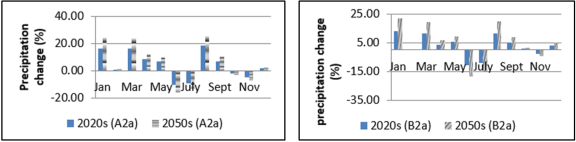
Figure 3. Percentage change in mean monthly precipitation of A2a and B2a scenarios.

Figure 3 shows the precipitation experiences a mean annul increase amount by 3.5% and 5.3% for A2a scenario at 2020s and 2050 respectively. But, the precipitation exhibits a mean annual decrease in amount by 2.55% and 4.36% for B2a scenario at 2020s and 2050s.

3.1.3. Projected Maximum Temperature

This Figure 4 depicts that the projected period will experience high increase in maximum temperature for both A2a and B2a scenarios. However, the increments will be less for B2a scenario relative to A2a scenario. This is due to the fact that A2a represents medium high scenario which produces more CO2 as compared to B2a scenario.

Download: Download full-size image

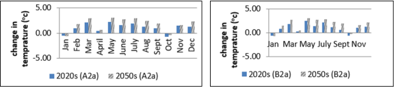
Figure 4. Maximum temperature A2a and B2a scenarios (delta values).

3.1.4. Projected Minimum Temperature

Figure 5 depicts the projected average monthly maximum temperature, minimum temperature positive change with respect to base period. The downscaled minimum temperature in 2020s indicated that the minimum temperature will rise by 1.1°C and 0.94°Cfor both A2a and B2 scenarios. For 2050s the increment will be 1.71°C for A2a and 1.54°C for B2a scenarios respectively.

Download: Download full-size image

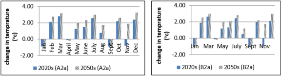
Figure 5. Change in average monthly minimum temperature A2a and B2a scenarios (delta values).

3.2. Watershed Delineation and Determination of Hydrologic Response Units

Lake Hawasa watershed was delineated, by dividing two sub-watersheds: the gauged (Tikur Wuha River) and un-gauged sub-watershed were delineated (Figure 6). The only gauged river in this watershed is the Tikur Wuha River and its catchment area based on SWAT delineation is 62317 ha. The un-gauged part of Lake Hawasa watershed has a catchment area of 59124 ha. That means, out of the total catchment only 51.3% is gauged and 48.7% is not gauged. After sub-watershed delineation, the determination of hydrologic response units (HRUs) was performed for which unique soil and land use combinations are within sub basins modeled together irrespective of their spatial positioning.

3.3. Hydrological Model Calibration, Validation and Uncertainty Analysis

Before calibration the parameter sensitivity analysis was done using the Arc SWAT interface for the gauged catchment at the outlet which is found near Dato. The parameters are ranked with decreasing sensitivity according to the mean relative sensitivity (MRS) of the parameters, and their category of sensitivity was also defined based on the

[20]

classification. Sensitivity is divided into four classes: small to negligible (0≤MRS<0.05), medium (0.05≤MRS<0.2), high (0.20≤MRS<1.0), and very high (MRS≥1.0).

The model result reveals that the most sensitive parameters considered for calibration were soil evaporation compensation factor, initial SCS Curve Number II (Cn2), available water capacity (Sol_Awc), Soil depth (Sol_Z), base flow alpha factor (Alpha_Bf), threshold depth of water in the shallow aquifer for “revap” to occur (Revapmn), groundwater "revap" coefficient (Gw_Revap) and average slope steepness in increasing sensitivity order.

Because of its simplicity SWAT CUP (SUFI-2 algorithm) was used for calibration, validation and uncertainty analysis of the SWAT model in Tikurewuha River. The period for calibration was having duration of six years (72 months) from January, 1990 to December, 1995; and the calibration was done using the most sensitive parameters.

Download: Download full-size image

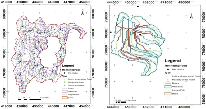
Figure 6. The Delineated sub basins for ungauged and gauged Sub watershed.

Table 3, Figures 7 and 8 show the calibration and validation results of the sub watershed, better correlation coefficient (R²) and the Nash-Sutcliffe (1970) simulation efficiency values show the very good agreement between the simulated and gauged monthly flows of the sub watershed. These values satisfied the recommendation made by Morasi et al. (2007), where R² and Nash- Sutcliffe efficiency (NSE) are expected to have values more than 0.6 and 0.5, respectively.

Download: Download full-size image

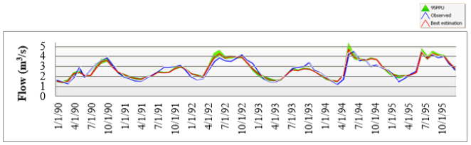
Figure 7. Calibration result of average monthly simulated and observed flow.

Accordingly, the result for flow calibration shows that 80% of the observed data is bracketed by the 95PPU (p-factor) and r-factor had a value of 0.27, which are good results. The smaller the r-factor, which quantifies the thickness of the 95PPU, the smaller the uncertainties and the better calibration work.

Download: Download full-size image

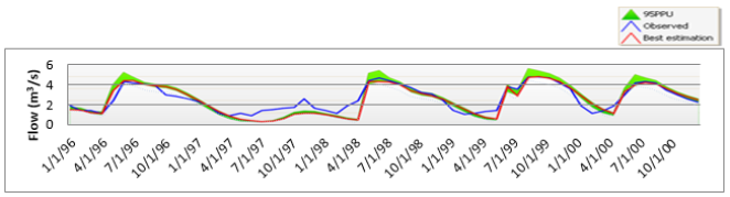
Figure 8. Validation result of average monthly simulated and gauged flow.

For the stream flow validation, 70% of the measured data were bracketed by the 95PPU while the r-factor had value of 0.3. Unlike the calibration, the flow simulation during validation is satisfactory with relatively large uncertainties. Generally the model is able to simulate with reasonable accuracy over the modeled period.

Table 3. Calibration and Uncertainty analysis results using SUFI2 for Tikurwuha River.

variable	P_factor	R_factor	R²	NSE
Flow (m³/s) Calibration period 1991-1996	0.8	0.27	0.88	0.88
Flow (m³/s) Validation period 1997-2000	0.7	0.3	0.84	0.78

Generally, the SWAT model performed well in simulating flows for calibration as well validation period based on calibrated parameters.

3.4. Projected Lake Water Balance Components

The water balance is estimated based on the inflow and the outflow (evaporation) of the Lake Hawasa. The inflow component is the summation of the over-lake precipitation and stream flow from gauged and un-gauged rivers and outflow component is the summation of the over-lake evaporation from the lake. In this study, lake water balance is established for the baseline period (1978-2000) and the two future time horizons 2020s and 2050s. The sum of the inflow from gauged and un-gauged catchments is used to estimate the total stream flow into the lake.

Table 4. Water balance components (10^6 m³) with expected percentage changes (%).

LWB components	Baseline	Scenarios	2020s	2050s
Gauge catchment inflow volume	86.28	A2a	89.92 (+4.22%)	91.57 (6.14%)
Gauge catchment inflow volume	86.28	B2a	88.37 (+2.42%)	89.86 (+4.15%)
Un-gauged catchment inflow volume	74.8	A2a	77.84 (+4%)	79.21 (+5.9%)
Un-gauged catchment inflow volume	74.8	B2a	76.5 (+2.35%)	77.8 (+4.03%)
Rainfall Over lake	80	A2a	84 (+3.5%)	85.6 (+5.3%)
Rainfall Over lake	80	B2a	82.6 (+2.55%)	84 (+4.36%)
Evaporation Over lake	153	A2a	156 (+1.64%)	159 (+2.64%)
Evaporation Over lake	153	B2a	155.5 (+1.5%)	158 (2.4%)
Storage change	87	A2a	95 (9%)	97.4 (11.9%)
	87	B2a	92 (5.7%)	93.7 (7.7%)

(+) indicates increase and (-) decreases of change in percentage

Generally, inflows to the lake, over-lake precipitation and evaporation will be expected to increase for both A2a and B2a emission scenarios.

Table 4 shows the annual distribution of hydrological variables considered for Lake water balance of the two scenarios (baseline, 2020s and 2050s) corresponding to climate change. Different scenarios produce a wide range of changes in the hydrological parameters. For the impact of climate change, most hydrological variables increased for the two time horizons. Precipitation falling over the lake will be expected to increase by 2.5% in 2020s and up to 5.3% in 2050s, inflow volume increased by 2.4% in 2020s and 6.14% in 2050s and evaporation over lake increased by 1.5% in 2020s and 2.64% in 2050s for both A2a and B2a scenario.

4. Conclusions

In this study, hydrological impact of climate change on Lake Hawasa water balance components were estimated in response to the A2a and B2a emission scenarios. SWAT has proved to be very well simulating the hydrological process of the watershed. The regression coefficient (R²) and the Nash-Sutcliffe efficiency (NSE) values obtained proved this fact. Based on the hydrological simulation carried out, more than 70% of the precipitation falling in the watershed is lost through evapotranspiration and it is more than six times the total flow. So, evapotranspiration can be more affected by the changing climate than any other hydrological component.

Generally climatic variables (i.e. precipitation and temperature) will be expected increase for both A2 and B2 future scenarios with an inflow to the lake.

This study should be extended by considering combined future (projected) changes in land use, soil and other climate variables in addition to the changes in precipitation and temperature and the outcome of this study is based on single GCMs of two emission scenarios (A2a and B2a). However, it is better to apply different GCMs and emission scenarios so as to make comparison between different models as well as to explore a wide range of climate change scenarios that would result in different hydrological impact. Hence, this work should be extended in the future by including different GCMs and emission scenarios.

Abbreviations

CUP	Calibration Uncertainty Program
GCMs	Global Circulation Models
HadCM3	Hadley Centre For Climate Prediction and Research Coupled Model
HRUs	Hydrologic Response Units
IPCC	Intergovernmental Panel On Climate Change
NSE	Nash- Sutcliffe Efficiency
SDSM	Statistical Downscaling Model
SWAT	Soil And Water Assessment Tool

Declaration

We declare that the manuscript titled " Modelling Hydrological Impact of Climate Change on Lake Hawassa Watershed, Southern Ethiopia " is original and has not been published or submitted for publication elsewhere. The contributions of the authors are as follows: the first author developed the concept, developed model and drafting manuscript; the second author contributed to the concept development, data collection and manuscript drafting; the third author has supervised this project and drafting manuscript and fourth author was responsible for concept development and drafting the manuscript. All authors have approved the final version of the manuscript.

Author Contributions

Wendmagegn Girma: Conceptualization, Methodology, Software, Validation, Visualization, writing - original draft, Writing - review & editing

Brook Abate: Conceptualization, Methodology, Writing - original draft, Writing - review & editing

Conflicts of Interest

The authors declare no conflicts of interest.

References

[1]	C. Change et al., “Climate Change 2007,” 2007.
[2]	R. Alley et al., “INTERGOVERNMENTAL PANEL ON CLIMATE CHANGE Climate Change 2007 : The Physical Science Basis Summary for Policymakers Contribution of Working Group I to the Fourth Assessment Report of the Intergovernmental Panel on Climate Change,” 2007.
[3]	A. H. Linde, J. C. J. H. Aerts, R. T. W. L. Hurkmans, and M. Eberle, “Comparing model performance of two rainfall-runo ff models in the Rhine basin using di ff erent atmospheric forcing data sets,” 2007.
[4]	M. D. Belete, “The impact of sedimentation and climate variability on the hydrological status of Lake Hawassa, South Ethiopia,” p. 145, 2013.
[5]	P. Qin et al., “Climate change impacts on Three Gorges Reservoir impoundment and hydropower generation,” J. Hydrol., vol. 580, Jan. 2020, https://doi.org/10.1016/j.jhydrol.2019.123922
[6]	B. Narsimlu, A. K. Gosain, B. R. Chahar, S. K. Singh, and P. K. Srivastava, “SWAT Model Calibration and Uncertainty Analysis for Streamflow Prediction in the Kunwari River Basin, India, Using Sequential Uncertainty Fitting,” Environ. Process., vol. 2, no. 1, pp. 79-95, 2015, https://doi.org/10.1007/s40710-015-0064-8
[7]	S. G. Setegn, D. Rayner, A. M. Melesse, B. Dargahi, and R. Srinivasan, “Impact of Changing Climate on Water Resources Variability in the Lake Tana Basin, Ethiopia,” 2010. Available: https://kth.diva-portal.org/smash/record.jsf?pid=diva2%3A294412&dswid=-8423
[8]	K. S. Abdo, B. M. Fiseha, T. H. M. Rientjes, A. S. M. Gieske, and A. T. Haile, “Assessment of climate change impacts on the hydrology of Gilgel Abay catchment in Lake Tana basin, Ethiopia,” vol. 3669, no. September, pp. 3661-3669, 2009, https://doi.org/10.1002/hyp
[9]	W. Girma and B. Abate, “Trend of Lake Evaporation Considering Climate Change, the Case of Lake Hawasa, Ethiopia,” Int. J. Sci. Res., vol. 3, no. 8, pp. 1605-1610, 2014. Available: https://www.ijsr.net/archive/v3i8/MDIwMTU1NQ==.pdf
[10]	C. Y. Xu, E. Widén, and S. Halldin, “Modelling hydrological consequences of climate change - Progress and challenges,” Adv. Atmos. Sci., vol. 22, no. 6, pp. 789-797, 2005, https://doi.org/10.1007/BF02918679.
[11]	R. L. Wilby and C. W. Dawson, “Using SDSM — A decision support tool for the assessment of regional climate change impacts User Manual,” no. October, pp. 1-64, 2001.
[12]	G. Di, P. Alam, and I. Kota, “Special Report on Emissions Scenarios,” 2011.
[13]	S. Neitsch et al., “A compilation of SWAT Model publications by Jeff Arnold, Raghavan Price of one set of SWAT book + DVD for countries in Tier A and Tier B (based on the World Bank), in US $ (The book is of A5 size, 415 pp., weighing approx. 450 g) TIER LIST Please,” vol. 1, 2009.
[14]	D. Shewangizaw and Y. Michael, “Assessing the Effect of Land Use Change on the Hydraulic Regime of Lake Awassa,” Nile Basin Water Sci. Eng. J., vol. 3, pp. 110-118, 2010.
[15]	J. Schuol and K. C. Abbaspour, “Advances in Geosciences Calibration and uncertainty issues of a hydrological model (SWAT) applied to West Africa # Ivory Coast VOLTA,” Adv. Geosci., vol. 2, pp. 137-143, 2006.
[16]	K. C. Abbaspour, M. Vejdani, and S. Haghighat, “SWAT-CUP calibration and uncertainty programs for SWAT,” MODSIM07 - Land, Water Environ. Manag. Integr. Syst. Sustain. Proc., pp. 1596-1602, 2007.
[17]	J. E. Nash and J. V. Sutcliffe, “River Flow Forecasting through Conceptual Models Part I - A discussion of Principles,” J. Hydrol., vol. 10, pp. 282-290, 1970.
[18]	V. Te Chow, D. R. Maidment, and L. W. Mays, Applied hydrology. 1988.
[19]	L. Z. Abraham, “Climate Change Impact on Lake Ziway Watershed Water Availability, by Climate Change Impact on Lake Ziway,” vol. 3, 2006.
[20]	T. Lenhart, K. Eckhardt, N. Fohrer, and H. Frede, “Comparison of two different approaches of sensitivity analysis,” vol. 27, pp. 645-654, 2002.

Cite This Article

Plain Text BibTeX RIS

APA Style

Girma, W., Abate, B. (2025). Modelling Hydrological Impact of Climate Change on Lake Hawassa Watershed, Southern Ethiopia. International Journal of Data Science and Analysis, 11(5), 143-152. https://doi.org/10.11648/j.ijdsa.20251105.13

Copy | Download

ACS Style

Girma, W.; Abate, B. Modelling Hydrological Impact of Climate Change on Lake Hawassa Watershed, Southern Ethiopia. Int. J. Data Sci. Anal. 2025, 11(5), 143-152. doi: 10.11648/j.ijdsa.20251105.13

Copy | Download

AMA Style

Girma W, Abate B. Modelling Hydrological Impact of Climate Change on Lake Hawassa Watershed, Southern Ethiopia. Int J Data Sci Anal. 2025;11(5):143-152. doi: 10.11648/j.ijdsa.20251105.13

Copy | Download

@article{10.11648/j.ijdsa.20251105.13,
  author = {Wendmagegn Girma and Brook Abate},
  title = {Modelling Hydrological Impact of Climate Change on Lake Hawassa Watershed, Southern Ethiopia
},
  journal = {International Journal of Data Science and Analysis},
  volume = {11},
  number = {5},
  pages = {143-152},
  doi = {10.11648/j.ijdsa.20251105.13},
  url = {https://doi.org/10.11648/j.ijdsa.20251105.13},
  eprint = {https://article.sciencepublishinggroup.com/pdf/10.11648.j.ijdsa.20251105.13},
  abstract = {Climate change refers to variations in the mean state of climate or variability of its properties such as rate, range and magnitude that extends for a long period due to external influences. The sign of climate change and its impact is revealing on different natural and manmade systems directly or indirectly. In this study, hydrological impact of climate change on Lake Hawassa water balance components was estimated in response to the A2a and B2a emission scenarios. Hydrological impact of climate change on Lake Hawasa water balance components were estimated in response to the A2a and B2a emission scenarios. Observed and future climatic variables were used to verify the hydrological impact. The future climate variables were predicted by using General Circulation Model (GCM) which is considered as the most used tool for estimating the future climatic condition. Statistical Downscaling Model (SDSM) was applied in order to downscale the climate variables to watershed level. Then, hydrological model soil and water analysis tool (SWAT) was applied to simulate the water balance components and calibrated by SWAT CUP (calibration uncertainty program) with sequential Uncertainty Fitting, Version 2 (SUFI-2) algorithm. The simulation result revealed that, by 2020s, the total average annual inflow volume into Lake Hawassa will rise significantly up to 6.14% for A2a and 5.9% for B2a-scenarios.
},
 year = {2025}
}

Copy | Download

TY  - JOUR
T1  - Modelling Hydrological Impact of Climate Change on Lake Hawassa Watershed, Southern Ethiopia

AU  - Wendmagegn Girma
AU  - Brook Abate
Y1  - 2025/10/09
PY  - 2025
N1  - https://doi.org/10.11648/j.ijdsa.20251105.13
DO  - 10.11648/j.ijdsa.20251105.13
T2  - International Journal of Data Science and Analysis
JF  - International Journal of Data Science and Analysis
JO  - International Journal of Data Science and Analysis
SP  - 143
EP  - 152
PB  - Science Publishing Group
SN  - 2575-1891
UR  - https://doi.org/10.11648/j.ijdsa.20251105.13
AB  - Climate change refers to variations in the mean state of climate or variability of its properties such as rate, range and magnitude that extends for a long period due to external influences. The sign of climate change and its impact is revealing on different natural and manmade systems directly or indirectly. In this study, hydrological impact of climate change on Lake Hawassa water balance components was estimated in response to the A2a and B2a emission scenarios. Hydrological impact of climate change on Lake Hawasa water balance components were estimated in response to the A2a and B2a emission scenarios. Observed and future climatic variables were used to verify the hydrological impact. The future climate variables were predicted by using General Circulation Model (GCM) which is considered as the most used tool for estimating the future climatic condition. Statistical Downscaling Model (SDSM) was applied in order to downscale the climate variables to watershed level. Then, hydrological model soil and water analysis tool (SWAT) was applied to simulate the water balance components and calibrated by SWAT CUP (calibration uncertainty program) with sequential Uncertainty Fitting, Version 2 (SUFI-2) algorithm. The simulation result revealed that, by 2020s, the total average annual inflow volume into Lake Hawassa will rise significantly up to 6.14% for A2a and 5.9% for B2a-scenarios.

VL  - 11
IS  - 5
ER  -

Copy | Download

Author Information

Wendmagegn Girma

Department of Civil Engineering, Addis Ababa Science & Technology University, Addis Ababa, Ethiopia

Contact Email

http://orcid.org/0009-0007-7606-6080
Brook Abate

Department of Civil Engineering, Addis Ababa Science & Technology University, Addis Ababa, Ethiopia

Download PDF

Submit an Article

Plain Text BibTeX RIS

APA Style

Girma, W., Abate, B. (2025). Modelling Hydrological Impact of Climate Change on Lake Hawassa Watershed, Southern Ethiopia. International Journal of Data Science and Analysis, 11(5), 143-152. https://doi.org/10.11648/j.ijdsa.20251105.13

Copy | Download

ACS Style

Girma, W.; Abate, B. Modelling Hydrological Impact of Climate Change on Lake Hawassa Watershed, Southern Ethiopia. Int. J. Data Sci. Anal. 2025, 11(5), 143-152. doi: 10.11648/j.ijdsa.20251105.13

Copy | Download

AMA Style

Girma W, Abate B. Modelling Hydrological Impact of Climate Change on Lake Hawassa Watershed, Southern Ethiopia. Int J Data Sci Anal. 2025;11(5):143-152. doi: 10.11648/j.ijdsa.20251105.13

Copy | Download

@article{10.11648/j.ijdsa.20251105.13,
  author = {Wendmagegn Girma and Brook Abate},
  title = {Modelling Hydrological Impact of Climate Change on Lake Hawassa Watershed, Southern Ethiopia
},
  journal = {International Journal of Data Science and Analysis},
  volume = {11},
  number = {5},
  pages = {143-152},
  doi = {10.11648/j.ijdsa.20251105.13},
  url = {https://doi.org/10.11648/j.ijdsa.20251105.13},
  eprint = {https://article.sciencepublishinggroup.com/pdf/10.11648.j.ijdsa.20251105.13},
  abstract = {Climate change refers to variations in the mean state of climate or variability of its properties such as rate, range and magnitude that extends for a long period due to external influences. The sign of climate change and its impact is revealing on different natural and manmade systems directly or indirectly. In this study, hydrological impact of climate change on Lake Hawassa water balance components was estimated in response to the A2a and B2a emission scenarios. Hydrological impact of climate change on Lake Hawasa water balance components were estimated in response to the A2a and B2a emission scenarios. Observed and future climatic variables were used to verify the hydrological impact. The future climate variables were predicted by using General Circulation Model (GCM) which is considered as the most used tool for estimating the future climatic condition. Statistical Downscaling Model (SDSM) was applied in order to downscale the climate variables to watershed level. Then, hydrological model soil and water analysis tool (SWAT) was applied to simulate the water balance components and calibrated by SWAT CUP (calibration uncertainty program) with sequential Uncertainty Fitting, Version 2 (SUFI-2) algorithm. The simulation result revealed that, by 2020s, the total average annual inflow volume into Lake Hawassa will rise significantly up to 6.14% for A2a and 5.9% for B2a-scenarios.
},
 year = {2025}
}

Copy | Download

TY  - JOUR
T1  - Modelling Hydrological Impact of Climate Change on Lake Hawassa Watershed, Southern Ethiopia

AU  - Wendmagegn Girma
AU  - Brook Abate
Y1  - 2025/10/09
PY  - 2025
N1  - https://doi.org/10.11648/j.ijdsa.20251105.13
DO  - 10.11648/j.ijdsa.20251105.13
T2  - International Journal of Data Science and Analysis
JF  - International Journal of Data Science and Analysis
JO  - International Journal of Data Science and Analysis
SP  - 143
EP  - 152
PB  - Science Publishing Group
SN  - 2575-1891
UR  - https://doi.org/10.11648/j.ijdsa.20251105.13
AB  - Climate change refers to variations in the mean state of climate or variability of its properties such as rate, range and magnitude that extends for a long period due to external influences. The sign of climate change and its impact is revealing on different natural and manmade systems directly or indirectly. In this study, hydrological impact of climate change on Lake Hawassa water balance components was estimated in response to the A2a and B2a emission scenarios. Hydrological impact of climate change on Lake Hawasa water balance components were estimated in response to the A2a and B2a emission scenarios. Observed and future climatic variables were used to verify the hydrological impact. The future climate variables were predicted by using General Circulation Model (GCM) which is considered as the most used tool for estimating the future climatic condition. Statistical Downscaling Model (SDSM) was applied in order to downscale the climate variables to watershed level. Then, hydrological model soil and water analysis tool (SWAT) was applied to simulate the water balance components and calibrated by SWAT CUP (calibration uncertainty program) with sequential Uncertainty Fitting, Version 2 (SUFI-2) algorithm. The simulation result revealed that, by 2020s, the total average annual inflow volume into Lake Hawassa will rise significantly up to 6.14% for A2a and 5.9% for B2a-scenarios.

VL  - 11
IS  - 5
ER  -

Copy | Download